Diodes: AC Analysis of Large Signals#
Input signal is large enough to move diode between multiple regions
Assume input signal is low frequency for now.
Input to Output Transfer Characteristic#
How to Analyze a Circuit to find the Transfer Characteristic#
We are, of course, focusing on circuits that contain diodes in this chapter. The following approach leads to the values you will need in order to develop the plot for the transfer characteristic
Assume reverse-bias
Write an expression for the voltage across the diode as a function of the input
Set the diode voltage equal to the value for which the diode should “turn-on”, aka become forward-biased
Solve for the value of input
Set the diode voltage equal to the value for which the diode should breakdown
Solve for the value of input
Write an expression for the circuit output as a function of the input
Assume forward-bias
Write an expression for the circuit output as a function of the input
Assume breakdown
Write an expression for the circuit output as a function of the input
Example: Half-wave Rectifier#
For a first example let’s consider a circuit that is common in many electronic devices. The first step in converting AC to DC is to remove the negative portion of a waveform. The half-wave rectifier is the simplest way to accomplish this.

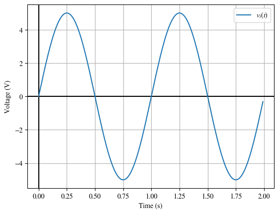
Developing the transfer characteristic allows us to answer the question: What is the output given an input signal? Let’s use this sine wave as input:
Let’s get started.
Assume Reverse-bias#

%% assume reverse-bias
clear all
close all
clc
format short eng
format compact

syms Va Vb vi
e(1)=Va==vi;
e(2)=0-(Vb/1e3)==0;
sol=solve(e,Va,Vb);
Vd=sol.Va-sol.Vb %diode voltage as function of input

Vrf=eval(solve(Vd==0.7,vi)) %border between rev/for
Vrb=eval(solve(Vd==-100,vi)) %border between rev/breakdown

Vout=sol.Vb-0 %output as function of input in reverse region
The output of this analysis:
input value corresponding to the diode transitioning between reverse and forward regions
input value corresponding to the diode transitioning between reverse and breakdown regions
expression of output in terms of the input for the reverse region
Assume Forward-bias#

%% assume forward-bias
clear all
close all
clc
format short eng
format compact

syms Va Vb vi
e(1)=Va==vi;
e(2)=Va-Vb==0.7;
sol=solve(e,Va,Vb);

Vout=sol.Vb-0 %output as function of input in forward region
The output of this analysis:
expression of output in terms of the input for the forward region
Assume Breakdown#

%% assume breakdown
clear all
close all
clc
format short eng
format compact

syms Va Vb vi
e(1)=Va==vi;
e(2)=Va-Vb==-100;
sol=solve(e,Va,Vb);

Vout=sol.Vb-0 %output as function of input in breakdown region
The output of this analysis:
expression of output in terms of the input for the breakdown region
Putting it all together#
Using the output of the analysis performed above, we can express the transfer characteristic in two forms:
1. Transfer Characteristic: Piecewise Function
2. Transfer Characteristic: Graphical Plot
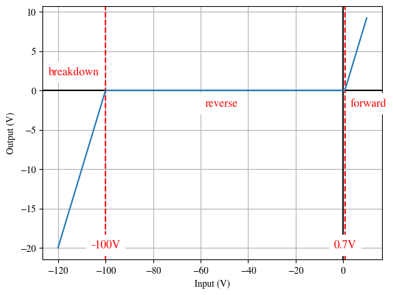
Take a moment to find how the outputs of the above sections are used to create both of these forms.
The voltages that are borders between regions show up as bounds in the piecewise function and vertical lines in the plot.
The output expressions are the values of the forms. They are expressed mathematically in the piecewise function and plotted over the correct domains in the plot.
Using the Transfer Characteristic to find a Time-Domain Response#
The transfer characteristic is just an intermediate result. We will use it, along with the input signal, to find the output.
I’ve included \(v_i(t)\) from the problem statement here. I have also transferred the border between the reverse and forward regions. Notice that while it was a vertical line in the transfer characteristic plot, here it is horizontal. Both indicate a value of \(v_i\). On the transfer characteristic \(v_i\) is represented on the horizontal axis. On the time-domain plot here, \(v_i\) is represented on the vertical axis.
I did not include the border between the reverse and breakdown regions here as the input signal does not cross that border.
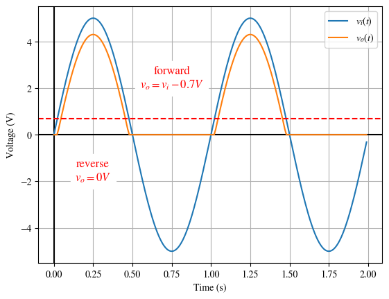
When the input is above the border (in the forward region) the output follows the expression found during the forward assumption analysis.
When the input is below the border (in the reverse region) the output follows the expression found during the reverse assumption analysis.
Example: Clipper #1#

Example: Clipper #2#
